Next: Part II: Mathematical Modelling Up: Mathematical Modelling and Simulation Previous: Introduction
Part I: Cardiovascular Risk Strategies in
Renal Transplantation
Kidney transplantation has revolutionised patient management with end stage renal disease and death
nowadays is more likely to be associated with premature cardiovascular (CV) complications. However, patient
survival is still depressed compared to the general population at large. In a retropsective study,
Woo et al (2001) [henceforth W01] estimated the graft and patient survival for a group of transplant
recipients attending treatment at the Western Infirmary Renal Unit in Glasgow. Additional to the standard
survival data contained in each patient record, W01 also tabulated a spectrum of cardiovascular risks
such as diabetes, high blood pressure, previous myocardial infarctions and electrocardiogram abnormalities.
A Cox proportional hazards model was then used to deduce the relative risks associated with each of the conditions
and to deduce the patient and graft survivor functions. The distribution of the patients across each risk-factor
is given in Table 1.
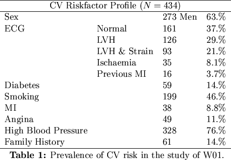
Currently in the UK, graft allocation is determined almost entirely by immunological and match criteria. However, CV risk has been shown (W01) to be an important prognostic variable in patient and graft survival. The question we have posed [McLean et al (2000), McLean & Jardine (2001)] is as to whether transplant allocation strategies based on CV risk would optimise total patient numbers. This has an obvious monetary implication for the health service as any increase in graft numbers, minimises patient time on haemodialysis which is very expensive.
What's the next step, though? It would be impossible to envisage running clinical trials to evaluate such strategies. We can, however, do the next best thing and appeal to simulations taking place in silico1. Discrete event simulation allows us to follow or simulate each patient as they arrive on the hospital system and move to and from the waiting list and transplanted list until death. Indeed, discrete event simulation has been used in a similar context in the past to evaluate potential patient numbers on waiting lists. See for example the work done by Davies & Davies (1987), Bolger & Davies (1992), Davies & Flowers (1994), Davies & Davies (1994) and Davies & Roderick (1998). However, those simulations were not driven by survivor functions derived from medical data but rather had their survivor functions taken as good guesses of trends in patient survival (they used classical exponential failure-time distributions). What was new in our study was that we used actual patient and graft survival functions and focussed on the outcome of varying CV strategies in renal transplantation.
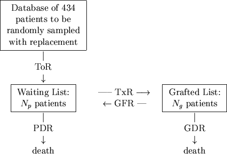
In terms of our model, depicted in Figure 1, patients arrive onto the simulation by randomly sampling records held on the database with replacement at the constant take-on-rate of ToR = 100 patients per year. These patients are placed onto the waiting list where they are randomly sampled at a transplant rate of TxR = 80/yr onto the grafted patient list. Thus far, no special sampling strategies based on CV risk-factors have been implemented. As patients arrive onto the waiting list, they are allocated a survival time2 based on their risk-factor profile and upon the fact that they have not yet been transplanted. Upon being transplanted, patients have their personal survival time updated to reflect the period of time they have waited and also their increased survival likelihood due to the transplant. Those transplanted patients are also assigned a graft survival time based on the graft survivor function. As simulated time progresses, hence, either a transplanted patient's graft will fail or the patient will die. If the former occurs, the patient simply moves back to the waiting list and has his or her personal survival time recalculated. However, should a patient die, then they are removed there and then from the simulation. At all times during the simulation, a count is kept of the number of waiting-list and transplanted patients and of the rates at which patients die or undergo graft failure. A sample simulation is shown in Figure 2.
 |
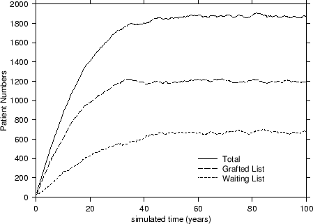 |
An interesting point to note is that each of the curves from Figure 2 attains an equilibrated or steady state value for the patient numbers after forty or so years. This value was used to characterise the standard simulation3 and also to compare it to other transplant strategies that we subsequently analysed. Of the various strategies based on cardiovascular risk considered, we were particularly interested in:
- the reduction of the acute rejection probability from its value today of ARP = 50% to a theoretically possible future value of 10% reflecting potential improvements in immunosuppresant drugs,
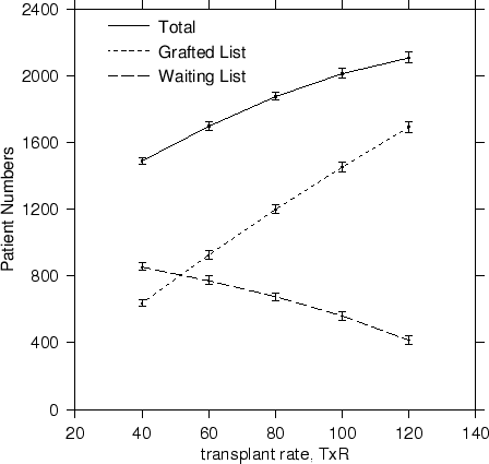
- the variation of the transplant rate between TxR = 40 to 120 patients per year reflecting an increase in the availability in cadaver kidneys, and
- both 100% and 50% reductions in the number of smokers and a preferential treatment strategy for the non-smokers.
These strategies were relatively straight forward to implement. In the case of reducing the number of smokers, for example, we simply altered our sampling with replacement subroutine to sample smokers at a lower rate. For preferential treatment to non-smokers, the software scanned the waiting list for non-smoker patients, transplanting them before transplanting smoker patients.
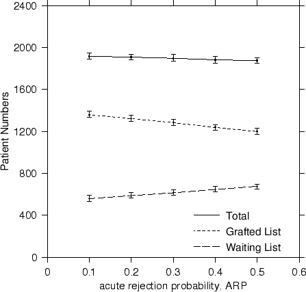 |
In terms of steady state results, a reduction in the likelihood of acute rejection saw a drop in the patient waiting list numbers from ~700 to ~600 patients, an increase in the number of transplanted patients from 1200 to 1350 for an overall increase in total numbers. Although this is to be expected, we have provided a coherent way of quantifying the actual patient numbers in a way not possible before. The trends are plotted in Figure 3.
For an increase in the availability of cadaver kidneys, the transplant rate TxR must increase. Increases in avaliability lead to an increase in transplanted patient numbers and to a decrease on the waiting list, for an overall increase in total numbers surviving. The trends are reproduced in Figure 4.
We considered the results from strategies aimed at reducing the number of smokers in terms of their percentage deviations from the standard reference simulation where no special strategy was implemented. Table 2 shows the percentage deviations from the standard simulation.
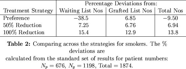
What is startling here is that although any absolute reduction in the number of smokers leads to increases on all the lists, a treatment based on preferential treatment to non-smokers fairs quite badly in comparison to the standard simulation. Here, grafted numbers are increased but waiting list numbers crash spectacularly and overall numbers are down, too. Preferential treatment strategies are thus ultimately detrimental to patient numbers.
Next: Part II: Mathematical Modelling Up: Mathematical Modelling and Simulation Previous: Introduction
